
Besides the table partitioning to improve performance and costs in BigQuery, there is also another technique available called clustering.
A little heads-up: Clustering and partitioning don’t preempt each other. And in most cases, it makes sense to use both in conjunction.
What are clustered tables?
Using clustered tables, BigQuery automatically organizes and colocates related data based on one or multiple selected columns. Important to note here is that the order of columns you are specifying for clustering is essential. But more on this later.
Since BigQuery does almost everything automatically –– in regards to clustering –– the only thing you have to do is to tell BigQuery on which columns and in which order you want BigQuery to cluster your data.
BigQuery then stores the data in multiple blocks inside the internal BigQuery storage. Storing the data in pre-sorted blocks means that BigQuery can –– based on your query filter clause –– use these blocks to prevent scans of unnecessary data.
According to the official docs using clustering will significantly improve performance when the scanned table –– or table partition –– exceeds 1 GB.
BigQuery offers automatic re-clustering, which means that even when you add new data to the tables, BigQuery will automatically sort them into the existing blocks.
A small example of a clustered table compared to a non-clustered one
You can see a table with randomly inserted data on the left side and an on the name and event column clustered table on the right side in the following image.
As you can see, rows with the same name are located right beneath each other. And in the range of the same name’s the rows with the same event are also colocated.
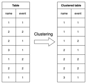
Taking this example, you can already imagine the possible improvement when querying data. As an example, let’s assume that you want to query all values where the name equals “1”.
Without clustering, BigQuery would have to scan the whole table because each row could contain the value “1” in its name column.
With clustering, BigQuery knows that only the first three columns will match this filter condition. That results in 50% fewer scanned columns since all the possible resulting rows are right beneath each other, and BigQuery can skip the other 50%. Also, 50% fewer checked rows also means 50% fewer costs since BigQuery charges you on the bytes read. Even though this might not be 100% accurate, as we will see later, it’s accurate enough to get the point of clustering data in tables.
The process of skipping specific blocks on scanning is also called block pruning. Even though BigQuery doesn’t necessarily create one block per one distinct value in the clustered column. The amount of blocks BigQuery creates depends highly on the amount of data stored. For 1 MB of data, even though it might contain 100 different values in the clustered column, BigQuery won’t create 100 blocks and save 99% of bytes read when filtering for one specific value. But the more (distinct) data is available inside the table; the more effective clustering will become. As already mentioned above, Google suggested a minimum table size of 1 GB to see significant improvements using clustering. But we will see in the next section that improvements will start way earlier.
Hands-On
Now it’s time for some actual hands-on coding and seeing some real-world examples. I split the hands-on part into four small portions.
- Easy script to create some test data we then can import and query.
- Import the test data into BigQuery as a normal and as a clustered table.
- Query both tables with the same query and compare results.
- Making an assumption on Google’s clustering block size based on a real example.
Create test data
We will orient ourselves by the first image in this article to create test data, where we showed how BigQuery organizes a clustered table compared to a normal one.
That means that we will have two columns. One column is representing a name, the other one representing an event.
Unlike the last article, we will dynamically create the data via a JavaScript script and write it into a CSV file. We need a minimum amount of data –– we will create 5,000,000 rows resulting in a 28 MB CSV file –– so we can see some effect of the clustering.
So, let’s check out the actual code for generating our test data.
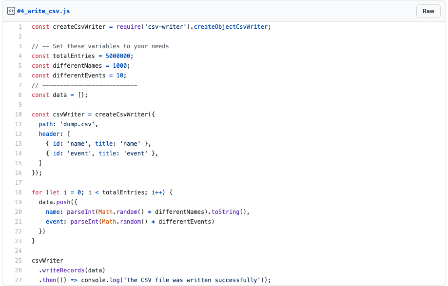
Code_csv#4
As you can see, we are using the csv-writer NPM module for writing the CSV file. So make sure you install it via npm i –save csv-writer before running the script.
The script itself should be easy to understand. First, we define some constants that determine the number of rows, amount of different names, and events that the script will generate randomly. Due to simplicity’s sake, I used plain numbers to represent the names.
When you use my default values, the script will produce a 28 MB CSV file containing exactly 5,000,000 rows of data – plus one additional for the column header – with 1,000 different names and ten different events. The script defines a name as a value between 0 and 999 and an event as a value between 0 and 9.
Of course, the produced CSV file will contain a little bit of different data each time you run it. But due to the high number of occurrences, you can expect each name to occur approximately 5.000 times.
Now that the test data is ready, it’s time to ship it to BigQuery.
Create a new table with data via CSV import
If you look at the following snippet, you will see many similarities to the last article’s CSV import script. And true, most of it is the same code. The main difference is the fourth parameter of the importCSV() method. Before we used timePartitioning, we now use clustering to define the fields that BigQuery should cluster.
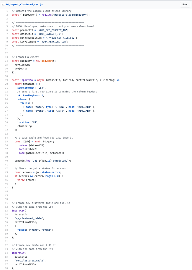
Code_Import-clustered_csv
In the script, we define the clustering fields as [“name”, “event”], which means BigQuery first clusters for the name and then for the event column.
After you run the script successfully –– it might take a bit to import the ~28 MB CSV file to BigQuery and wait for the clustering to finish –– we can verify via the CLI if BigQuery added clustering correctly.
bq show –format=prettyjson
YOUR_GCP_PROJECT:YOUR_DATASET_ID.my_clustered_table
This command will print the metadata of your BigQuery table to the CLI. There you should find some entry for clustering looking like the following:
“clustering”: {
“fields”: [
“name”,
“event”
]
},
If you run the same command for the non_clustered_table, you should not see any entry for clustering.
Run queries on the imported data
Now that we imported all the data to the normal and the clustered table and verified that BigQuery enabled the clustering correctly on our clustered table, it’s time to run some queries against it to compare their statistics.
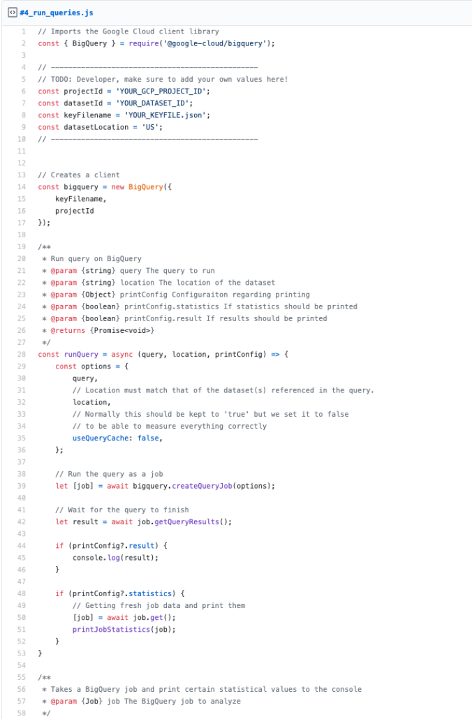
Again, we are using quite a lot of code from the previous article because most of it is independent of any clustering or partitioning.
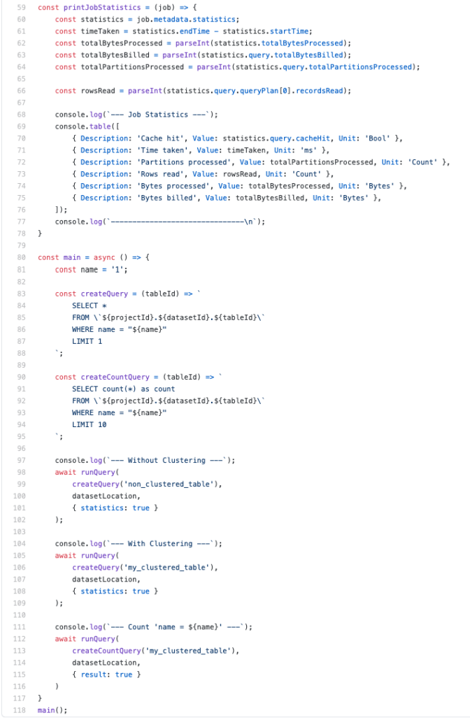
Compared to before, we added some printConfig to our runQuery method to define what it should print — either the query result or the job statistics, or both.
In our standard search query – createQuery – we are filtering the rows by a specific name with the value “1”. In theory, this should affect around 5,000 rows because we have created 5,000.000 rows with 1,000 different names resulting in approximately 5,000 entries per name.
We added one additional query – createCountQuery – that we will run and print its result. We run this query to verify our assumption that around 5.000 rows should be affected by our filer condition.
Query results
When you run the above script, you should get a similar result to the following:
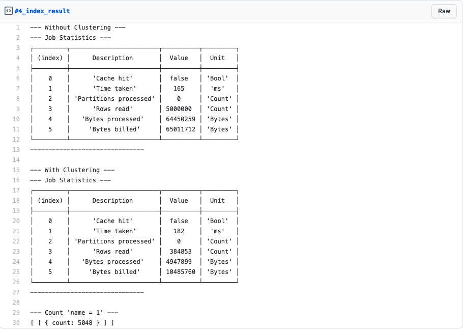
Because we don’t have a lot of data here, the Time taken is similar in both queries. As explained in the beginning, significant performance improvements will be visible when approaching the table size of 1 GB and more.
But what you can see is that the Rows read and the Bytes processed – which Google charges you for – has significantly decreased.
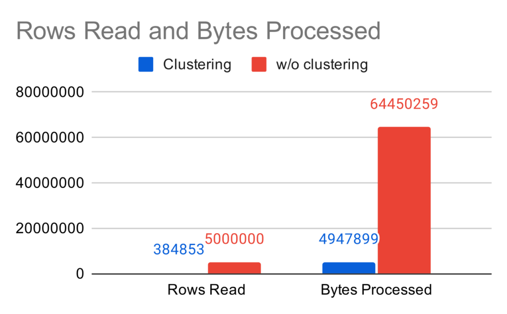
From 5,000,000 rows read and 64,450,259 bytes processed, we decreased down to 384,853 rows read and 4,947,899 bytes processed. That is a theoretically cost saving of 92.3%! Just because we used clustering.
You can also see this big difference in the following graph:
Rows-Read-and-Bytes-Processed
The attentive audience will also notice that the Bytes billed are not 92.3% smaller, even though one could expect this. And yes, absolutely right. But that is because Google charges a minimum of 10 MB per query regardless of the actual bytes processed. When the Bytes processed are higher than 10 MB, the Bytes billed will be almost always the same as the Bytes processed.
Google’s clustering block size, an assumption
Besides this, you might also notice that the Rows read count is way higher than the 5,000 rows we expect to only scan for our query. That is due to some Google internal configuration of BigQuery where a cluster range’s minimum size exists. Even though Google’s “magic” is not only about the plain size of the colocated data.
You could assume that when you increase the amount of data up to a certain point, the Rows read should have the same value as the affected rows. Since we saw above that even though only 5,000 rows should be affected – the query read 384,853 rows – we could think that somewhere around this value, there could be some “magic number”.
As a small example – I don’t want to go too deep into this topic yet – I changed our above test data set like the following:
- I increased the total entries to 10,000,000.
- I decreased the different names to 20.
These changes should, in theory, result in 20 different names, each occurring approximately 500,000 in the table. With this in place, we have more occurrences than the query from before has rows read.
So let’s check the result:
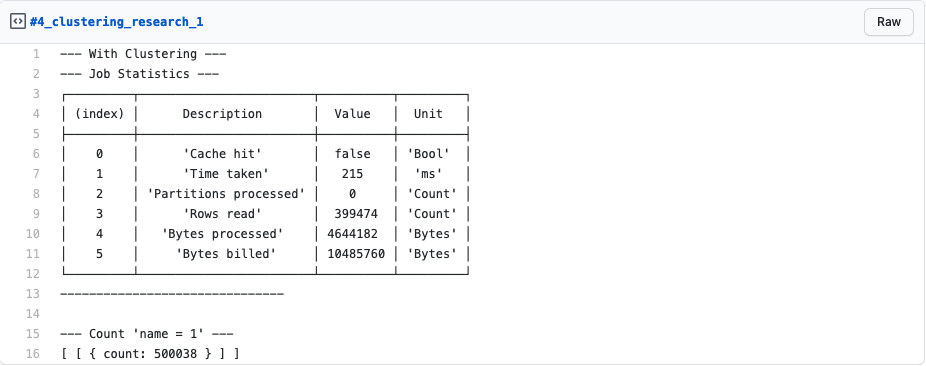
At first glance, the result might look somewhat confusing. Even though we now have 500,000 entries that match our filter criteria, BigQuery just read close to 400k rows? And we also verified with our createCountQuery that there are really around 500k rows matching our filter.
But wait! If you remember, we are using a LIMIT 1 in our query because we were never interested in the actual result but only looked at the job statistics.
Let’s change this LIMIT 1 to a LIMIT 600000, so we are retrieving all affected rows and look again at the results of our script:

We can now clearly see that the job read a total of 799,675. That pretty close to two times the read rows of the LIMIT 1 case, which is 798,948. There might be something there…
Even though I haven’t found any official documentation, it might provide you some hints regarding the possible block size for clustered tables. But this is purely my investigation so far, and there are for sure also other factors involved. I want to move this even further, but I think that would be too much for this article’s scope since it should be rather some introduction to clustering and not a deep dive into its internal structures.
Clustering limitations and common pitfalls to be aware of
Maximum number for clustered columns –– BigQuery supports up to four columns for clustering.
Clustering of string types –– When you use string types for clustering, it’s essential to be aware that BigQuery only uses the first 1,024 characters of the cell value for clustering. Everything beyond that limit will not be considered by BigQuery’s clustering algorithm even though it’s valid to have longer values written into the cells.
Order of clustered columns –– The order in which you define the columns for clustering is essential for good performance. If you want to benefit from the clustering mechanism, it’s necessary to use all the clustered columns or a subset of them in the left-to-right sort order in your filter expression. If you have the clustered columns A, B, and C, you will have to filter for all three of them, just A, or A and B. Just filtering for B and C will not result in the expected performance boost. As a best practice, you should always specify the most frequently filtered or aggregated column first. The order in the actual SQL filter expression doesn’t affect the performance. It’s just essential on which columns you are filtering.
What’s next?
After we now know how we can stream, load, and query data in BigQuery and use partitioned and clustered tables to improve our performance and reduce costs, we will learn how to set up scheduled queries and typical use cases in the following article.
Author
Pascal Zwikirsch
Pascal Zwikirsch is a Technical Team Lead at Usercentrics. He manages a cross-functional team of several frontend and backend developers while providing a seamless connection between the technical world and the product managers and stakeholders.
Pascal was a former frontend developer for several years and now specializes in backend services, cloud architectures, and DevOps principles. He experienced both worlds in detail. This experience and the collaboration with product managers made him capable of constructing full-fledged scalable software.
Besides his job as a Team Lead of the B2B developer team, he likes to share his in-depth knowledge and insights in articles he creates as an independent technical writer.
For more content, follow me on LinkedIn
Join our growing community of data privacy enthusiasts now. Subscribe to the Usercentrics newsletter and get the latest updates right in your inbox.