
Especially when working with Big Data, costs can quickly explode, and performance can degrade fast when data starts to pile up.
BigQuery offers the possibility to create partitioned tables that helps to prevent exploding costs and decreasing performance.
Of course, the use case has to fit the idea behind partitioning even though most Big Data use cases should fit there in one or another way.
Google provides three different ways to partition BigQuery tables:
Ingestion Time — Tables are partitioned based on the time they ingestion time.
Time-unit column — Tables are partitioned based on a time-unit column. Valid values here are TIMESTAMP, DATE, and DATETIME.
Integer ranged — Tables are partitioned based on an integer column.
Read about Big data marketing now
What is time-unit partitioning, and how does it work?
Easy put partitioning a table is like splitting up the table into several “sub”-tables. Each of these partitioned tables has its unique key for easy and fast access.
When using partitions, you can run your queries only on a specific set of the partitioned tables and thus are saving many rows your query doesn’t have to iterate to check for your conditions.
Using “time-unit column” partitioning in BigQuery works like the following:
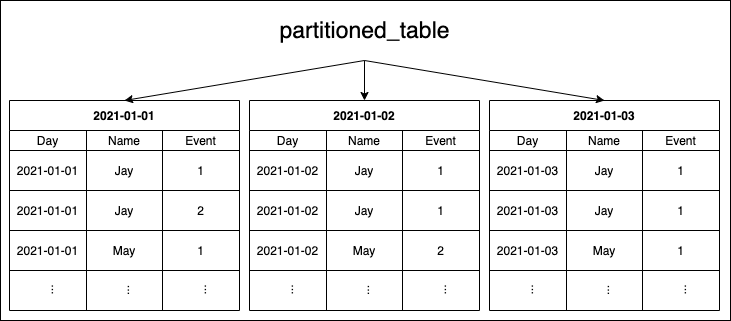
You specify a column of your table with the type TIMESTAMP, DATE, or DATETIME and how granular the partitions should be. Valid values here are hourly, daily, monthly, and yearly. If you choose daily, all partitioned tables will each contain all rows of a specific day, so you can quickly get all rows or filter the rows for a particular day without running through ALL the other partitioned tables.
Assuming that you write at least one entry per day over one year (365 days) and are using daily partitioning, you will have 365 partitioned tables at the end of the year. That is because each partition reflects one day of data.
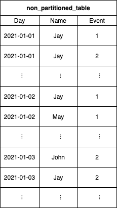
You can see a “normal” non-partitioned table and right afterward the same table with a daily partition on the “Day” column in the following two images.
Keep in mind that making actual use of the partitioning, your queries will also have to reflect it. For example, it doesn’t benefit when you have your table partitioned by a date column but then not filtering for the date, which results in a full table scan again.
How much can it improve costs/performance?
Now that we went over the basics, one of the most crucial questions is “How much can it improve costs/performance?”. No answer fits all use cases but let’s provide an example you can use as a blueprint for your calculations.
To get to some concrete values, let’s assume the following:
- You use daily partitioning since you have to query data either on one day or a day range.
- You already have six years’ worth of data resulting in ~2190 days / partitioned tables.
- You evenly distributed your data across all the days (of course, somewhat unlikely, but we have to make an assumption here).
- The total size of your data is 72 TB -> 12 TB per years -> 1 TB per month -> ~33 GB per day
For non-partitioned tables, your queries will always have to do a full table scan resulting in 7,2e+13 Bytes (72 TB) to be processed and billed on each query.
Example #1: Running a query on one particular day
Requesting data only for one specific date means that the query can access the needed partition directly and process this one partition but doesn’t have to process the other 2189.
Above, we assumed that one day/partition contains around 3,3e+10 (33 GB) of data. That means we would only process ~0.046% (33 GB / 72,000 GB or 1 / 2190) of the whole dataset resulting in a 99.954% reduced usage in data and thus costs!
Example #2: Running a query for a 30-day range
Requesting a 30-day range is analogous to the above example and can be simplified to 30 / 2190 => 1.37%. Even though that is way more as in example #1, it is still a reduction of 98.6% in size and thus costs compared to a full table scan!
Actual costs of the examples:
Now let’s see what the above example queries would cost each compared to a non-partitioned table. Google charges $5.00 per TB according to their official pricing docs resulting in the following values.
Non-partitioned table: $5.00 * 72 TB = $360.00
Example #1: $5.00 * 0.033 TB = $0.165
Example #2: $5.00 * 0.99 TB = $4.95

The difference is pretty stunning, right?
Of course, partitioning will increase the performance proportional to the cost reduction. When the query has to evaluate 99% fewer rows, you can imagine that it needs around 99% less time to finish.
Why you save even more money with partitioning
Even though the above examples are already a super hefty cost reducer, there is even more to it when we think about the second cost driver in BigQuery. Storage costs.
As already mentioned in the first article, BigQuery has the concept of active and long-term storage. While Google charges only half for long-term storage, no disadvantages are coming with it. The only criterion is that there is no modification of the table data for at least 90 days. When you use partitioned tables, each partition is considered separately in regards to long-term storage pricing.
Let’s take our above assumptions regarding data size ( 33 GB per day) and distribution ( evenly ) and check its storage costs. Also, we further assume that in the last 90 days, we added some data every day.
This assumption results in the non-partitioned table never reaching the long-term storage status since there are daily changes to the table. On the other hand, the partitioned table always has just 90 partitions in the active storage and the remaining 2100 ones in the long-term one.
For active storage, Google currently charges $0.02 per GB for the location US (multi-region).
Non-partitioned table: $0.02 * 33 GB * 2190 = $1445.40 per Month
Partitioned table: $0.02 * 33 GB * 90 days + $0.01 * 33 GB * 2100 days = $59.40 + $693.00 = $752.40 per Month

As you can see, with partitioning, you can not only improve your on-demand analysis costs significantly but also reduce the storage costs by a lot.
Hands-On
Now let’s do some hands-on on some actual implementation and analyze the query results.
Since we already handled the setup of a Node.js BigQuery project in the last article , we won’t repeat it here. I also expect a globally initialized variable called ‘bigquery’ to exist in the following code snippets and that a BigQuery dataset is available.
We first have to create both tables with the same data set for comparing some actual — even though relatively small — non-partitioned table with a partitioned table.
Creating new tables with data from a CSV file
For this example, I prepared some CSV file containing ~72k of rows in the following format: dump.csv
date,name,event
2021-01-04 00:00:00.000000,Adam,4
2021-01-01 00:00:00.000000,Tom,2
2021-01-02 00:00:00.000000,Jay,1
2021-01-03 00:00:00.000000,Jay,3
….
The first row ‘date’ will be of the type DATETIME and thus in the following format: YYYY-MM-DD HH:MM:SS[.SSSSSS]
The actual values are not that important; I just made sure that I have four different dates mentioned there, so BigQuery creates four partitions I can later query accordingly. I then named the CSV file ‘dump.csv’ and added it beneath my script file ‘importCSV.js’, which content you can see in the following code snippet.
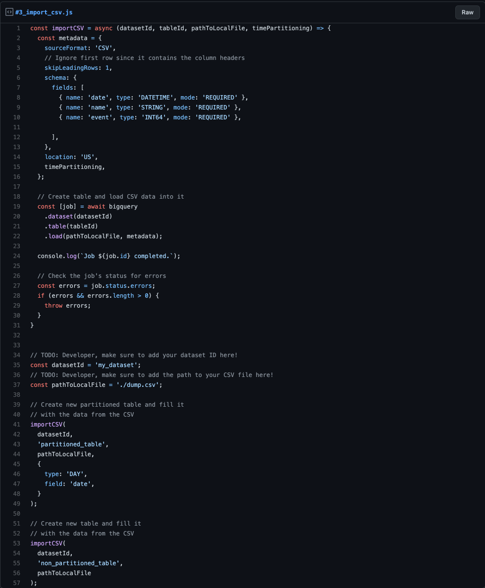
Code – import csv
The ‘importCSV()’ method in the above snippet is similar to what you should know from the previous article. The difference is that instead of calling some ‘createTable(…)’, we are referencing the ‘table(…)’ and then loading initial data together with some schema definition via the ‘load(…)’ method into it.
The “partition-specific” part of the ‘importCSV’ method is only the ‘timePartitioning’ variable passed into the function.
When you check the object, the script passes in for this parameter; it is pretty straightforward. We define the type as ‘DAY’, telling BigQuery that it should create daily partitioned tables. Also, via the ‘field’ property, we command BigQuery that it should use the column called ‘date’ as the partition column. You can find the official docs for the ‘TimePartitioning’ object here.
After we ran the above script and have created the two tables, we can now run and compare our queries with the following snippet.
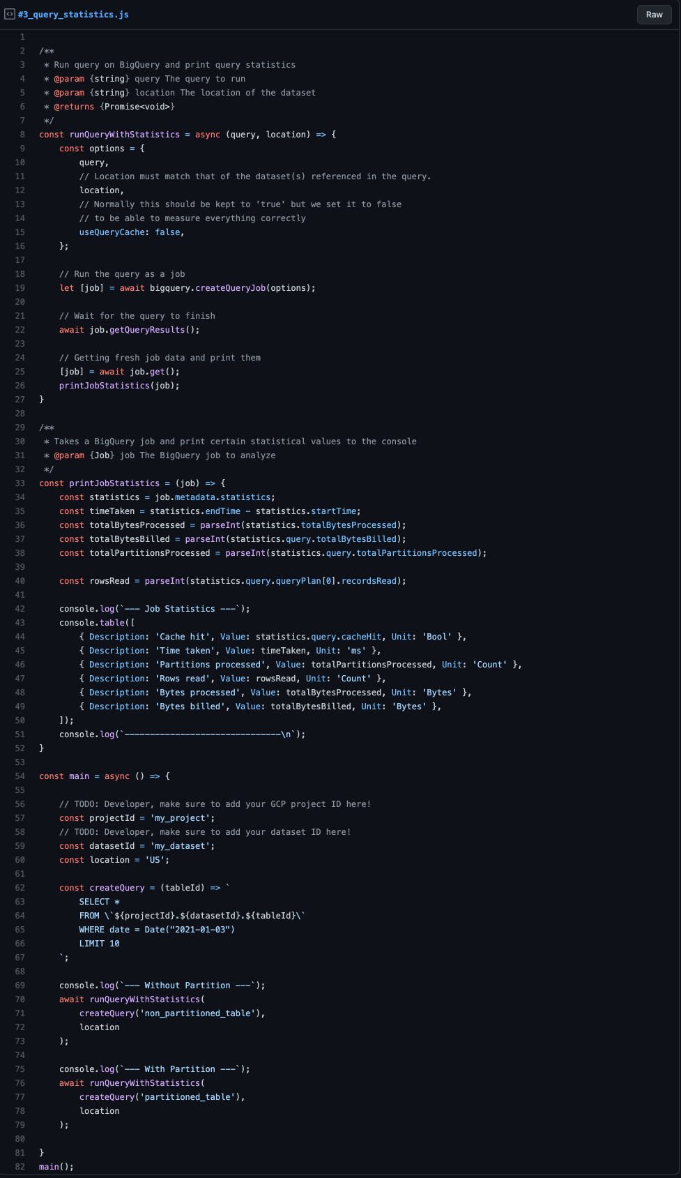
Query statistics
The script is kept very simple. In the ‘runQueryWithStatistics()’, we run the provided query and afterward pass the finished job to some method that prints the job statistics to the console. The critical part here is that we set ‘useQueryCache: false’ so BigQuery doesn’t use any caching in the background. That is important as we can’t compare metrics when served by cache. Of course, you should always keep this flag on ‘true’ — the default — when running in production!
The ‘printJobStatistics()’ method is even more simple. It more or less only accesses certain relevant properties and prints them to the console. We will discuss the individual metrics a bit later.
Let’s move further to the ‘main()’ method. Here the variables and a helper method for creating our query are defined. The ‘createQuery()’ only takes the ‘tableId’ as the input parameter to generate the same query for the non-partitioned and partitioned table that only differs by the referenced table.
Afterward, we run the ‘runQueryWithStatistics()’ method. Once on the ‘non_partitioned_table’-table and once on the ‘partitioned_table’-table and log the results.
You can see the output of the above script in the following snippet.
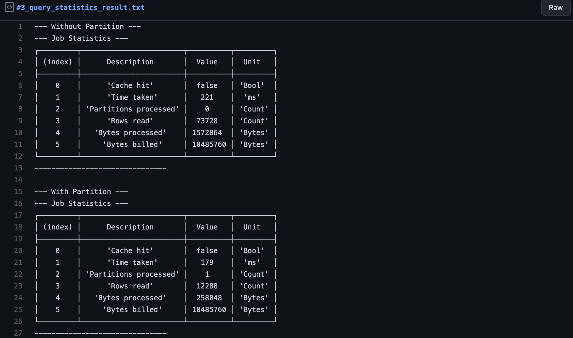
QUERY STATISTICS RESULT
Understanding the statistics
Now that we have the job statistics, we have to understand and interpret them accordingly to verify our assumptions.
Cache hit — This value only tells us that the cache wasn’t hit, and we can be sure that we didn’t receive a cached result that tamper with our metrics.
Since we explicitly set the cache to be disabled, this should always be ‘false’. If it appears to be ‘true’, something is wrong.
Time taken — Defines the time it took to run the query from its start till the end time.
Here we can see that the partitioned table is a bit faster (~19%). Based on my experience, I can say that this isn’t meaningful in our example since we are still in the milliseconds’ range and having only around 2 MB in data. Here side effects take a too big part in the time taken compared to the actual query.
This metric becomes significant if you reach several seconds or minutes of query processing time.
Partitions processed — Indicates how many partitions the query read. In the case of non-partitioned tables, this is always 0.
In our partitioned table’s output, we can see that it only read one partition since only one specific date was being queried and not a date range.
Rows read — How many rows the query had to read to finish.
Here we can already see that the two variants strongly differ. We have ~73k rows in the non-partition table case and only ~12k rows in the partition table. The rows read are already reduced by ~83.6%, reflecting in the following metric, “bytes processed”.
Bytes processed — The number of bytes the query had to process.
Similar to “rows read”, we can see an apparent reduction in size here. While the non-partitioned query has to scan the full ~1.6 MB of data, the partitioned one only had to process ~0.26 MB resulting in a reduction of ~83.4%.
Bytes billed — The number of bytes Google is charging you for this query.
Normally one would now expect that the “bytes billed” would also differ by around 83%. But the alert reader will notice that the values are the same.
This first unexpected behavior has a relatively simple origin. When checking the pricing details page of BigQuery you will find the following quote:
“… with a minimum 10 MB data processed per query.”
In our case, where we only process 1.6 MB and 0.26 MB in our two queries, Google rounds up the costs to a minimum of 10 MB of bytes billed, reflecting it in our statistics.
In the case of actual data, when you have several GB, TB, or even PB, the “bytes billed” will significantly differ and behave proportionally to the “bytes processed”.
Partitioning quotas and common pitfalls to be aware of
The maximum number of partitions — Using partitioning on BigQuery tables, there is a hard limit of 4,000 partitions per partitioned table.
Example:
When you are using daily partitioning on your table, you can cover at most 4,000 days (10.96 years) of data. Writing data for more days into the table will result in errors or rejections on BigQuery’s side.
Even though it’s unlikely that you run into this very fast with daily partitioning, using hourly partitioning, you will run into it after approximately 5.47 months.
Streaming data into partitioned tables — When streaming data into partitioned tables, one could expect that BigQuery adds the data immediately to the correct partition. Unfortunately, that is not true. BigQuery will first write streaming data to a temporary partition called ‘__UNPARTITIONED__‘ while the data is in the streaming buffer. Currently, there is no way to flush this buffer manually. Thus you have to wait till BigQuery automatically flushes this buffer after a certain amount of unpartitioned data is available or after a certain amount of time has passed. Google doesn’t provide any exact numbers regarding the mentioned amounts.
Even though when running the BigQuery command:
‘bq show –format=prettyjson YOUR_GCP_PROJECT:DATASET_ID.TABLE_ID‘
You can check the properties ‘estimatedBytes’ and ‘estimatedRows’ on the ‘streamingBuffer’ object to see how many bytes and rows are currently in the streaming buffer.
Require partition filter — When working with partitioned tables, it is always good practice to enable the ‘requirePartitionFilter’ flag for the partitioned table when creating it. Having this flag in place, BigQuery will always demand a predicate filter on the SQL query that tries to access the table. This flag helps prevent queries that would accidentally trigger a full table scan instead of accessing a particular partition or set of partitions and would result in high costs.
Don’t ‘OR’ your partition filter — One might think it’s enough to have the partitioned column in his SQL statement’s filter condition. Even though using ‘OR’ will still trigger a full table scan, it doesn’t need the partition filter to match.
Example:
Will trigger a full table scan:
WHERE (partition_column = “2021-01-01” OR f = “a”
Won’t trigger a full table scan:
WHERE (partition_column = “2021-01-01” AND f = “a”
As a best practice, I always advise to have the partition filter condition isolated and then ‘AND’ it with the actual filters you want to apply to the rows. That also helps to prevent wrong/expensive queries.
Example:
WHERE partition_column = “2021-01-01” AND ( ALL_THE_OTHER_CONDITIONS )
What’s next?
In the following articles, we will learn how to create and work with clustered tables in BigQuery to improve performance even further.
Author
Pascal Zwikirsch
Pascal Zwikirsch is a Technical Team Lead at Usercentrics. He manages a cross-functional team of several frontend and backend developers while providing a seamless connection between the technical world and the product managers and stakeholders.
Pascal was a former frontend developer for several years and now specializes in backend services, cloud architectures, and DevOps principles. He experienced both worlds in detail. This experience and the collaboration with product managers made him capable of constructing full-fledged scalable software.
Besides his job as a Team Lead of the B2B developer team, he likes to share his in-depth knowledge and insights in articles he creates as an independent technical writer.
For more content, follow me on LinkedIn
Join our growing community of data privacy enthusiasts now. Subscribe to the Usercentrics newsletter and get the latest updates right in your inbox.